Describe a situation in your research area where you would expect to see an interaction between continuous independent variables in a regression model.

In the preceding discussion of the effects of frequency and length on reaction time, I was making one big oversimplifying assumption. I was assuming that the relationship between frequency and RT (i.e., the fact that higher-frequency words are responded to faster, and how much faster this is) stays the same across words of different lengths.
That might not be true, however. We could imagine other scenarios. For example, maybe for long words there is a big effect of frequency, but short words are responded to fast no matter how frequent they are. Maybe high-frequency words have a positive effect of length (i.e., among high-frequency words, long words take longer to respond to than short words do) but low-frequency words have a negative effect (i.e., among low-frequency words, long words are responded to faster than short words). There are lots of possibilities you could imagine. These scenarios are interactions (see the ANOVA module for a more in-depth discussion of main effects and interactions).
The graph below shows the regression plane for the same set of data we have been discussing, only now I have included an interaction in my regression model. You can see how this changes the result: the plane is now slightly twisted. For high-frequency words, there is the expected length effect (long words are responded to more slowly than short words). On the other hand, for low-frequency words, length doesn't matter much; low-frequency words are responded to pretty slowly no matter what their length is. The interaction here is very subtle, but if you look closely you should be able to see it.
Formally, a model like this is accomplished by including another coefficient for the interaction between frequency and length. An example is shown in the formula below. . While the frequency coefficient (\(b_1\)) is multiplied by the frequency of a word (\(X_1\)), and the length coefficient (\(b_2\)) is multiplied by the length of the word (\(X_2\)), the interaction coefficient (\(b_3\)) is multiplied by the product of the frequency and length (i.e., frequency times length: \(X_1\times{}X_2\)):
The logic underlying this formula is not something you need to know for this class (although, as an exercise for yourself, you are welcome to try to figure out how this produces the abovementioned interaction effect—a good start would be to try drawing different regression lines for different values of length or different values of frequency), but it's useful to understand this so you can "plug in" values, like we did before, to predict reaction times. In practice, when you do actual regression analysis, coefficients can become difficult to understand (especially three-way interactions or even higher-order interactions); often the easiest way to understand the model is to plug the values into the formula and make one or more graphs, to see what the regression model looks like.
As I mentioned before, we rarely actually make these kinds of spinning three-dimensional graphs in reality; they're just not practical (for example, you can't print them out; plus, they're hard to read, and can't go beyond 3 dimensions). What's more common is to represent these kinds of data with multiple graphs. For example, I could make multiple graphs, each showing the effect of frequency on RT for words of a certain length. This allows me to see how the effect of frequency on RT for short words might be different than the effect of frequency on RT for long words:
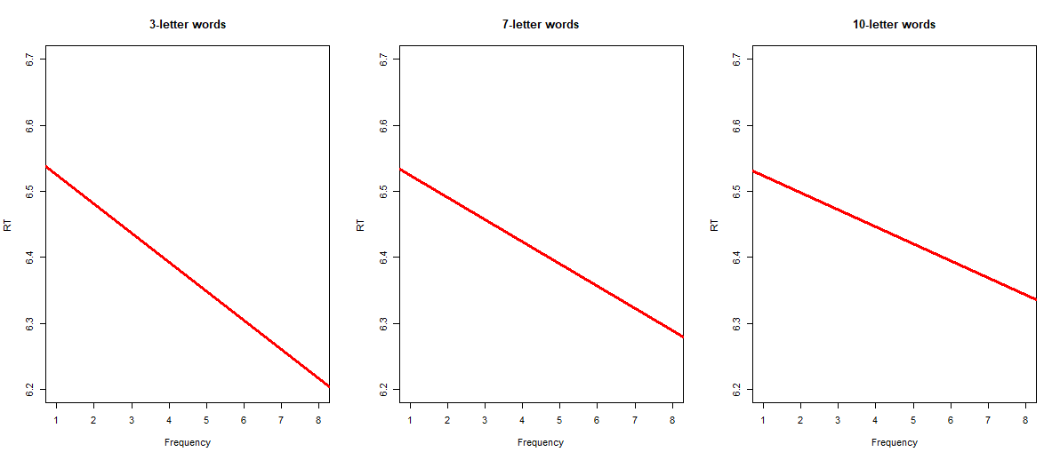
For a real-life example of this approach, see the figures 7, 9, and 11 in Lee et al. (2013). For example, in the bottom half of Figure 7, you can see that F0 influences perception of sounds with short VOT, but not of sounds with medium or long VOT. (You may also notice that the regression lines in these figures are curvy, not straight. How to make curvy regression lines is an extra regression concept that is beyond the scope of this module, but you will learn about it if you take a full class on regression.)
Describe a situation in your research area where you would expect to see an interaction between continuous independent variables in a regression model.
When you have finished these activities, continue to the next section of the module: "Categorical independent variables".
by Stephen Politzer-Ahles. Last modified on 2021-05-16. CC-BY-4.0.